PARADOX Hadoop user guide
This article gives a tutorial introduction to MapReduce parallel computing approach, and how it can be done on SCL’s hadoop cluster.
![]()
Introduction
The usual way in which we create parallel programs for PARADOX cluster is using MPI. The problems we solve that fit well with that approach, are the ones where the main bottleneck is processing power. Complexity of the simulation or a model being executed is much bigger than the relative size of dataset it runs on. However, you may have experienced problems where the sheer size of data is so large that filesystem access times become the dominant factor in the total execution time.
Years ago, Google had similar problem in indexing all the pages on the WWW. They also used commodity hardware which was heterogeneous, connected with a relatively slow network and prone to random hardware failures. To cope with all that they formalized the MapReduce approach.
This approach works on data sets wich consist of data records. The idea is to define the calculation in terms of two steps - a map step and a reduce step. The map operation is applied to every data record in the set and it returns a list of key-value pairs. Those pairs are then collected, sorted by key and passed into the reduce operation, which takes a key and a list of values associated with that key, and then computes the final result for that key, returning it also as a key-value pair.
In terms of unix commands, this is equivalent to the following:
where the mapper program (or script) takes each line of the input file, splits it into records according to its own rules, and derives one or multiple key-value pairs from it. It then outputs those key-value pairs to standard output which is then piped to sort for sorting. Reducer program takes sorted key-value pairs, each on a separate line on standard input, and performs a reduction operation on adjacent pairs which have the same key, outputing the final result for each key to its standard output.
This can be only one step of the analysis wich can go through as many iterations of map-reduce as needed.
Of course, not all problems can easily fit into the map-reduce framework, but for those that do, paralellization and reliability concerns are decoupled from the problem being solved. If any of the mappers or reducers fail, they will be restarted on a replica of the data chunk in question, possibly on some other data node. Also the system will scale the paralellism of the run according to available resources and distribution of the data set chunks on the data nodes.
To explore this approach further, we will first cover the distributed file system which underpins Hadoop and makes its operations efficient.
HDFS
Hadoop uses HDFS, a specialized filesystem, to acheve its parallel file acces and redundancy. This distributed file system keeps data split into chunks and redundantly spread across data nodes. Name node keeps the file system metadata, such as the directory layout, file attributes and also the mapping of which file chunks reside on which data node.
The size of a chunk can be specified on creation, but by default it is 64 MB. The number of replicas is also configurable, and it defaults to 3. This means that each file uploaded to HDFS is split into a number of chunks which are copied a number of times accross data nodes. These redundant copies help not only with fault tolerance, they are also used when parallel execution of map-reduce tasks needs to operate on a particular chunk. Having multiple copies on different data nodes enables the system to choose the least busy data node with the target chunk to execute the operations.
To interact with HDFS, we use the hdfs dfs commands, which mimic the standard Unix shell file commands, such as ls, chown, etc.
A user’s home directory is located on the /users/USERNAME path. It can be listed by executing:
The default directory for most commands, if an absolute path is not provided, is that user’s home directory.
Another commonly used command is to create a directory on the HDFS:
To upload some data onto HDFS one can use the put command:
To fetch data off the HDFS, use the get command:
Copying a dataset to HDFS from a remote location
One common issue a user with a lot of data could face is how to copy the data from a remote location onto the HDFS. This could be done by first copying the data onto the local file system of the head node, but that space is limited, and it’s an unnecessary step.
To directly copy a data from another machine which supports ssh access, one can execute on that machine:
To check the amount of free space on the HDFS use:
Also, the following command gives a report about the state of HDFS which includes the amount of free space:
Hadoop
Apache Hadoop is an open-source implementation of a distributed MapReduce system, with an entire ecosystem of other services built on top of it, such as distributed databases, data mining and machine learning execution environments, etc.
Since version 2, a Hadoop cluster is organized around the YARN resource manager. This resource manager is made to support uses more general than MapReduce, but for the purposes of this tutorial, we will focus only on concepts relevant to running distributed MapReduce steps.
A Hadoop cluster consists of a name node and a number of data nodes. The name node holds the distributed file system metadata and layout, and it organizes executions of jobs on the cluster. Data nodes hold the chunks of actual data and they execute jobs on their local subset of the data.
Users define their jobs as map, reduce and optionally combine functions which they submit for the execution, along with the locations of input and output files, and optional parameters regarding the number of reducers and similar.
Hadoop was developed in Java and its primary use is through Java API, which will be described in the next section. However, since Java has fallen behind in popularity for data science related fields, Hadoop also offers a “streaming” API, which is more general and it can work with map-reduce jobs written in any language which can read data from standard input and return data to standard output, which is basically any language. In this tutorial we will provide examples in Python.
MapReduce
MapReduce in Hadoop can run in several configurations. The most basic one is to run just one reducer in the reduce step. Even in this basic setting we can see quite a few terms in the picture below that we should explain.
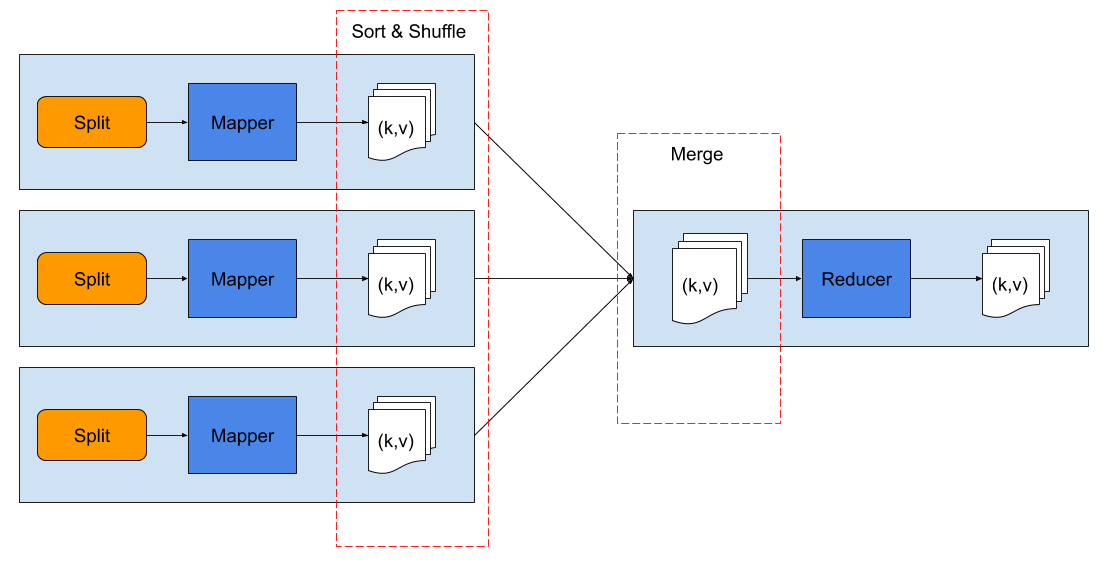
Each orange split box in the figure represents one chunk of input data, stored in HDFS. Mapper is the map function that is supplied in the job definition, and it is applied to every record in its local split (chunk). Mapper returns a list of key-value pairs it computes from the input records. Mapper can return zero, one or more key-value pairs from a single input record.
The returned key-value pairs are sorted by key and collected and merged from all the mappers to a single reducer. The reducer gets this input as key-values pairs, where values for each key are all the values from the map step that were associated with that key.
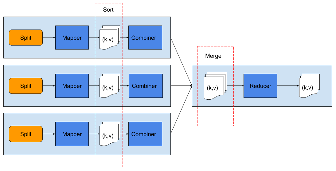
As the size of data returned from the map step can be quite large, to speed up the reduce step, Hadoop allows us to define a combiner function, which runs after each mapper finishes its chunk, and it processes the local data from that mapper. The combiner can be thought of as a local reduce step before sending data to the global reducer that will perform reduction on the complete key-values data returned by all the mappers.
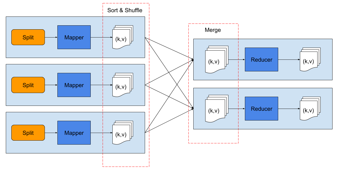
For cases where data is so large that it is too much for a single reducer to handle, multiple reducer can be launched in the reduce step.
Java API
Initially, Hadoop was developed as a part of open source search engine project (Nutch), and it was developed in Java which is its primarily supported language.
Since Java is a systems programming language with focus on large and complex systems, starting up a new project to develop for Hadoop, can be an involved process. To automate the project setup, we provide a maven archetype.
To use the archetype, you will need Java Development Kit (JDK), and maven already installed. Both are available on hadoop login node, but if you need to develop locally, most popular Linux distributions have OpenJDK and maven packages available, and on MacOS you can use Homebrew to install them. For Windows, please check out OpenJDK and Maven project sites for latest installers and installation instructions.
Once the prerequisites are there, the first step is to clone the archetype, and install it into the local maven registry via the following command:
After this you can switch to the directory where the project will be located, and execute the following command to create the project from the archetype:
The command will present you with a wizard that guides the creation of the project, requiring the following information:
- groupId - in maven terms this is the identifier of your group, usually it is your web domain name in reverse, such as for
www.scl.rsit would bers.scl - package - this is the Java package, usually it is left the same as groupId
- artifactId - the name of the project, for our test we used
mrtest
This is the layout of the project directory that we end up with:
mrtest/
├── pom.xml
└── src
    ├── main
    │   └── java
    │       └── rs
    │           └── scl
    │               └── App.java
    └── test
        └── java
            └── rs
                └── scl
                    └── AppTest.java
This archetype creates the standard wordcount example for MapReduce, which counts the frequency of words in a body of text. For test data, we can download some books from Project Gutenberg, and place them into a directory in HDFS. Assuming we’re in the directory where the text files (*.txt) are, we can use the following commands (lines staring with $) to upload our input files to the HDFS:
$ hdfs dfs -mkdir books

$ hdfs dfs -put *.txt books
2020-11-29 22:29:28,008 INFO sasl.SaslDataTransferClient: SASL encryption trust check: localHostTrusted = false, remoteHostTrusted = false
2020-11-29 22:29:28,769 INFO sasl.SaslDataTransferClient: SASL encryption trust check: localHostTrusted = false, remoteHostTrusted = false
2020-11-29 22:29:29,488 INFO sasl.SaslDataTransferClient: SASL encryption trust check: localHostTrusted = false, remoteHostTrusted = false

$ hdfs dfs -ls books
Found 3 items
-rw-r--r--   1 petarj supergroup     174693 2020-11-29 22:29 books/11-0.txt
-rw-r--r--   1 petarj supergroup    1276201 2020-11-29 22:29 books/2701-0.txt
-rw-r--r--   1 petarj supergroup     451046 2020-11-29 22:29 books/84-0.txt
After these commands, the dataset will be placed to /user/<USERNAME>/books, which in this case is /user/petarj/books since the user we are running these tests with is petarj. Your experiments will require to replace <USERNAME> with your username.
To build this project, execute: mvn package in the project directory. A lot of output will be echoed, but it can be ignored if the last few lines show BUILD SUCCESS in green letters. The interesting output is located in the target/mrtest-1.0-SNAPSHOT.jar file. It is the binary that will be executed by Hadoop to perform our wordcount analysis.
We can execute this analysis with the following command:
This command will produce a lot of output, which abreviated should look like the following:
2020-12-01 10:50:20,993 INFO client.RMProxy: Connecting to ResourceManager at hadoop/147.91.84.40:8032
...
2020-12-01 10:50:22,664 INFO mapreduce.Job: The url to track the job: http://hadoop:8088/proxy/application_1606692341173_0003/
2020-12-01 10:50:22,665 INFO mapreduce.Job: Running job: job_1606692341173_0003
2020-12-01 10:50:28,786 INFO mapreduce.Job: Job job_1606692341173_0003 running in uber mode : false
2020-12-01 10:50:28,789 INFO mapreduce.Job:  map 0% reduce 0%
2020-12-01 10:50:32,882 INFO mapreduce.Job:  map 67% reduce 0%
2020-12-01 10:50:33,893 INFO mapreduce.Job:  map 100% reduce 0%
2020-12-01 10:50:37,928 INFO mapreduce.Job:  map 100% reduce 100%
2020-12-01 10:50:38,952 INFO mapreduce.Job: Job job_1606692341173_0003 completed successfully
2020-12-01 10:50:39,125 INFO mapreduce.Job: Counters: 54
    File System Counters
...
The output of this run will be placed in /user/<USERNAME>/wordcounts directory, as per parameters of the run. The directory specified as the output, will contain an empty _SUCCESS file, if the run was successful, and a number of files containing key-value results from the reduce step. They will be named part-r-XXXXX where the XXXXX represent the number of each result part, as there can be more than one of them.
You can use commands like cat, head or tail in hdfs to quickly take a look at contents of the files like so:
$ hdfs dfs -head wordcounts/part-r-00000
# first 20 lines of output...

# or
$ hdfs dfs -tail wordcounts/part-r-00000
# last 20 lines of the file...

# or
$ hdfs dfs -cat wordcounts/part-r-00000
# contents of the entire file...
To fetch the results file from the HDFS you can use the hdfs dfs -get command mentioned in the previous section on HDFS.
Streaming
If you prefer to use languages other than Java, Hadoop offers the streaming API. The term streaming here refers to the way Hadoop uses standard input and standard output streams of your non-java mapper and reducer programs to pipe data between them. Relying on stdin and stdout for this enables easy integration with any other language.
The general syntax of the command to run streaming jobs is the following:
In the first example, we will reimplement the wordcount given above in Java, and this will demonstrate just how elegant a streaming solution can be. We could define our mapper in just a few lines of python:
This mapper will read text from standard input and for each word it will echo that word and the number 1 as the number of times the word appeared. The reducer will take those key-value pairs and sum the number of appearances for each word:
#!/usr/bin/env python3
import sys

prevWord = ''
prevCount = 0
for line in sys.stdin:
    word, count = line.split()
    count = int(count)
    if word == prevWord:
        prevCount += 1
        continue
    else:
        if prevWord != '':
            print(prevWord, prevCount)
        prevWord = word
        prevCount = 1
if prevWord != '':
    print(prevWord, prevCount)
The reducer is a bit more complicated as it must keep track of which key it is reducing on. This happens because it will get all the values for a single key on a separate key-value line, i.e. hadoop streaming mechanism won’t automatically collect all the values for a key into an array of values. However, even with this hinderance, the code is still quite concise.
If we assume the same input of Project Gutenberg books is in the same location /user/<USERNAME>/books, our example can be run like this:
The input and output parameters specify the locations for input and output data on the HDFS. Mapper and reducer parameters specify the mapper and reducer programs respectively. The following file parameters specify files on the local file system that will be uploaded to Hadoop and made available in the context of that job. Here we specify our python scripts in order to make them available for execution on the data nodes.
PageRank example
If the word count examples seem too simplistic, or you would like to see how a more involved analysis could be performed using MapReduce on Hadoop, in this section we will show how a popular analysis on graph (network) data could be performed.
The example task will be to calculate the PageRank of twitter users based on data of who follows whom on that social network. The datset used is available from Stanford SNAP as Twitter follower network. It contains a directed graph of Twitter users (from 2010) which has 1 468 364 884 edges between 41 652 230 nodes.

image credit: Wikipedia
PageRank will rank these users, giving the ranking of users by their “influence”. The rough idea is that the more followers a node has, the more influential it is, and the more those followers are influential, the more they contribute to the influence of the node they follow. A more in depth coverage of the algorithm can be found on the Wikipedia article and the original paper.
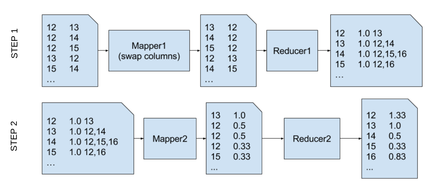
The dataset we use, originaly comes as an edge list with two integer user IDs per line, signifying that user with the second ID follows the user with the first ID. Since the MapReduce implementation of PageRank we use, expects the graph to be represented as an edge list, we will perform the analysis in two steps. The first mapper reverses the two user ID columns. So we get key-value pairs which signify that user ID 1 follows user ID 2. This is then reduced to the following record format:
| Key (user ID) | Current PageRank | List of followed IDs |
|---|---|---|
| 12 | 1.0 | 13 |
| 13 | 1.0 | 12, 14 |
| … | … | … |
In other words, our value is the current PageRank (1.0) and the list of follower IDs.
The mapper in the second step splits the key’s current PageRank value and contributes it to each of the users it follows. The second reduction just sums the contributed PageRanks for each of the followed nodes. This is graphically shown in the next figure:
The following listing show our implementation of the 2 steps described above.
File mapper1.py:
#!/usr/bin/env python3

import sys

for line in sys.stdin:
    target, follower = line.split()
    print('%d\t%d' % (int(follower), int(target)))
File reducer1.py:
#!/usr/bin/env python3

import sys

curr_user = None
curr_adjl = []

for line in sys.stdin:
    usr, adj = line.split()
    if usr == curr_user:
        curr_adjl.append(adj)
    else:
        if curr_user:
            print('%s\t%s' % (curr_user, '1.0 '+','.join(curr_adjl)))
        curr_user = usr
        curr_adjl = [adj]

if curr_user:
    print('%s\t%s' % (curr_user, '1.0 '+','.join(curr_adjl)))
File mapper2.py:
#!/usr/bin/env python3

import sys

for line in sys.stdin:
    key, pr, adj = line.split()
    pr = float(pr)
    adj = adj.split(',')
    cpr = 1.0*pr/len(adj)
    for t in adj:
        print('%s\t%f' % (t, cpr))
    print('%s\t%f' % (key, pr))
File reducer2.py:
#!/usr/bin/env python3

import sys

ckey = None
csum = 0.0

for line in sys.stdin:
    key, pr = line.split()
    pr = float(pr)
    if key == ckey:
        csum += pr
    else:
        if ckey:
            print('%s\t%f' % (ckey, csum))
        ckey = key
        csum = pr

if ckey:
    print('%s\t%f' % (ckey, csum))
We can place these scripts into a directory on the Hadoop login node (hadoop.ipb.ac.rs), and we get the following project directory layout:
twitterrank/
├── mapper1.py
├── mapper2.py
├── reducer1.py
└── reducer2.py
The input data is already uploaded to HDFS and is available at /user/petarj/twtest/twitter-2010.txt. With all that ready, we can launch the first MapReduce step with the following command:
This command will execute the step and create its output in the twit1 directory in the current user’s HDFS home directory (i.e. /user/<USERNAME>/twit1). This output will be the input for our next step which we launch with the following command:
This final step will store the output in /user/<USERNAME>/twit2 directory and we can -get it to our local file system or we can take a look at it directly on HDFS with the following command:
$ hdfs dfs -head twit2/

100000  0.000469
10000000    0.139423
10000003    1.816303
10000006    1.272653
10000009    2.431107
1000001 1.301035
10000012    1.001732
10000015    1.038887
10000018    1.862444
10000021    1.731199
10000024    2.610371
10000027    5.113444
10000030    3.792091
10000033    0.501711
10000036    1.000000
10000039    1.242241
...
This will show first 50 lines or so, of output which is of the format UserID PageRank. The entire analysis took about 1 hour and 12 minutes, which is about four times faster than what we measured running the serial analysis with the same map and reduce scripts on a single machine, and without any parallelization (except what we get from using unix sort and other commands). If you have the data on a local machine (e.g. in twtest/twitter-2010.txt file), you can test the serial run with the following commands:
$ cat twtest/twitter-2010.txt | ./mapper1.py | sort | ./reducer1.py > step1.dat
$ cat step1.dat | ./mapper2.py | sort | ./reducer2.py > step2.dat
On our 4 core test machine and a mechanical HDD, it took about 4 hours. To make our MapReduce analysis even faster we can increase the number of reducers, using the -D mapreduce.job.reduces parameter like in the following example, which launches 2 reducers per step:
$ mapred streaming -D mapreduce.job.reduces=2 -input /user/petarj/twtest/twitter-2010.txt -output mr_twit1 -mapper mapper1.py -reducer reducer1.py -file mapper1.py -file reducer1.py

$ mapred streaming -D mapreduce.job.reduces=2 -input /user/<USERNAME>/mr_twit1 -output mr_twit2 -mapper mapper2.py -reducer reducer2.py -file mapper2.py -file reducer2.py
The following calls launch 3 reducers per step:
$ mapred streaming -D mapreduce.job.reduces=3 -input /user/petarj/twtest/twitter-2010.txt -output 3r_twit1 -mapper mapper1.py -reducer reducer1.py -file mapper1.py -file reducer1.py

$ mapred streaming -D mapreduce.job.reduces=3 -input /user/<USERNAME>/3r_twit1 -output 3r_twit2 -mapper mapper2.py -reducer reducer2.py -file mapper2.py -file reducer2.py
Note: In the runs above, we’ve used different names for each run’s output directories since Hadoop would prevent us from rewriting old resulsts if the output path on HDFS already exists
The measured wall time for each of the runs above is given in the following table and histogram:
| run | wall time |
|---|---|
| serial | 4h 7m 54s |
| mapreduce (1 reducer) | 1h 11m 14s |
| mapreduce (2 reducers) | 33m |
| mapreduce (3 reducers) | 24m 15s |
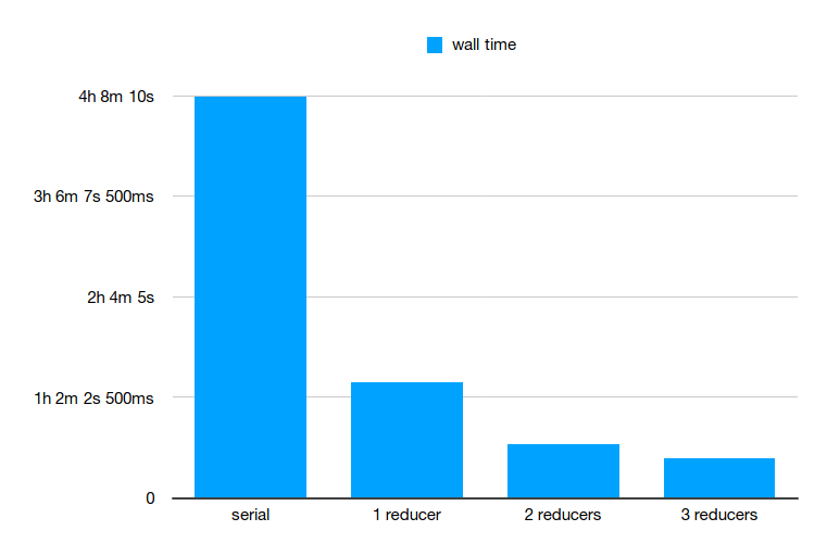
These measurements show how much speedup we can get from MapReduce on our Hadoop cluster with 3 data nodes. Unfortunately, because of the data semantics, this analysis does not lend itself to more speedup using combiner in our step, but other problems could expect even more speedup if they can include it.
We hope these examples have inspired you to try to formulate your solutions in MapReduce terms and made analysis on even greater datasets feasible.